If you add Excel increase/decrease indicators with a Custom number format code in Format Cells, you can put ▲ in front of positive numbers and ▼ in front of negative numbers, and even change their color, while leaving the cell values untouched. A format code splits positive, negative, and zero sections with semicolons, and in each section you write symbols in quotation marks and colors in square brackets. When you want to put the change inside a sentence, use the TEXT function, and when you need icons by range, use icon sets in conditional formatting.
"If only there were an arrow in front of each number showing whether it went up or down from last week, it would be so much faster to read." When you build a weekly ad report or a sales comparison table, the change column is often just a string of numbers like -1,250 and 3,400, and you end up checking the minus signs one by one. But if you type ▲ into each cell by hand, the numbers turn into text and you can no longer total them. In this post, I'll walk through how to add Excel increase/decrease indicators with custom formats, how to read format codes, and when to use the TEXT function or icon sets instead, based on Microsoft's official help.
1. Why Use a Custom Format for Increase/Decrease Indicators?
Because a number format only changes how a value looks, not the value itself. Microsoft's help explains that applying a number format only changes how the number is displayed and doesn't affect the cell value used in calculations, and that you can see the actual value in the formula bar. So even with a ▲▼ format applied to your change column, there's no problem totaling it with SUM or referencing it in other formulas.
I found this difference easy to understand by thinking of it as a sticker on a window. The number behind the glass stays as it is; you're just putting a ▲ sticker on in front of it and peeling it off again, so changing the sticker doesn't change the number itself. On the other hand, if you type "▲1,250" directly into a cell, you haven't added a sticker; you've turned the number itself into text, so it drops out of calculations.
To use a custom format, open the Format Cells dialog by clicking the small arrow (dialog box launcher) in the Number group on the Home tab or by pressing Ctrl+1, choose Custom in the Category list, and then write your code in the Type box that appears.
So what should you write in that box, and how?
2. How Do You Read a Custom Format Code?
A format code consists of up to four sections separated by semicolons (;), applied in order to positive numbers, negative numbers, zero, and text. For increase/decrease indicators you use the first three sections. Here's a summary of the rules set out in the help article.
- Number of sections: If you write only one section, it applies to all numbers; if you write two, the first section is used for positive numbers and zero, and the second for negative numbers.
- Symbols and text: Some symbols such as $, +, -, parentheses, and spaces are displayed as is, but any other characters must be wrapped in double quotation marks or preceded by a backslash (
\). For ▲▼, just wrap them in quotes, like"▲". - Colors: Put the color name in square brackets at the very start of the section. There are 8 colors you can use: Black, Green, White, Blue, Magenta, Yellow, Cyan, and Red.
- Placeholders:
0displays zeros to fill in missing digits, while#doesn't display insignificant zeros. Putting a comma between placeholders, as in#,##0, gives you a thousands separator.
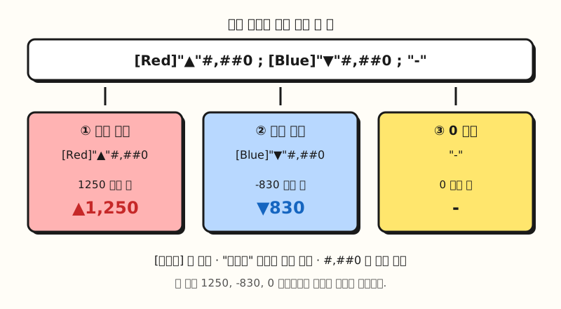 Split a single format code at its semicolons and you can set a different look for positive numbers, negative numbers, and zero (figure labels in Korean).
One confusing point is how color names are written. The English help writes them in English, like [Red] and [Blue], while the Korean help writes [빨간색] and [파란색] in the same place.
The color names Excel accepts may differ depending on its language version, so if you get an error when you enter one, I recommend first choosing a format in the Number category that shows negative numbers in red, and then moving to Custom. The help article also suggests picking one of the built-in formats as a starting point and editing it, so you can simply copy the color name already written in the Type box.
3. How Do You Add ▲▼ Arrow Codes in Excel?
Select the column that holds the change values (for example, column D, which subtracts last week from this week), go to Ctrl+1 > Custom, and enter one of the codes below in the Type box.
| Value to display | Format code | How it looks |
|---|---|---|
| Change in quantity or amount | [Red]"▲"#,##0;[Blue]"▼"#,##0;"-" | 1250 → ▲1,250 (red), -830 → ▼830 (blue), 0 → - |
| Percentage change | [Red]"▲"0.0%;[Blue]"▼"0.0%;0.0% | 0.125 → ▲12.5%, -0.04 → ▼4.0% |
| Symbols only, no color | "▲"#,##0;"▼"#,##0;"-" | Colors stay as they are; only arrows are added |
I left the minus sign out of the negative section because ▼ already says it's a decrease. Just as the Microsoft help example $0.00" Surplus";$-0.00" Shortage" writes the minus sign directly in the negative section, the look of the negative section is determined by exactly what you write in the code. If you want the minus sign to appear along with ▼, enter it like [Blue]"▼"-#,##0.
The % in the percentage-change code multiplies the value by 100 and displays it with a percent sign, so the cell must contain a ratio like 0.125, not 12.5.
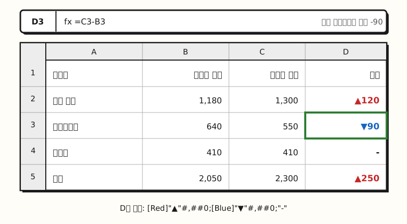 Example figure: the values in column D are still plain numbers; only the ▲▼ and colors are applied with a custom format (sample data, figure labels in Korean).
You can insert the ▲▼ symbols by clicking Symbol in the Symbols group on the Insert tab. The help article explains how to insert a symbol by typing its code in the Character code box at the bottom of the dialog; ▲ is Unicode 25B2 and ▼ is 25BC. It's handy to insert the symbol into a blank cell, copy it, and paste it inside the quotation marks in the Type box. If your team reads increases as blue and decreases as red, just swap the color names in the two sections.
But what if you want to put the change inside a sentence, like "Conversions ▲120" in the first line of a report?
4. Can You Build In-Sentence Indicators with the TEXT Function?
Yes, just put the same format code into the TEXT function. The TEXT function uses the structure TEXT(value, format_text) to convert a number into text in the format you want, and the format code must be wrapped in double quotation marks.
For example, if the change value is in D2, you can write ="Conversions "&TEXT(D2,"\▲#,##0;\▼#,##0;-"). The backslash (\) in front of ▲▼ means "display the next single character as is." Unlike in the Format Cells dialog, the whole code is already inside double quotation marks, so a backslash is used instead of quotes. You can also copy a code from the Custom list in the Format Cells dialog and paste it into the TEXT function.
There are two things to keep in mind, though.
- Colors don't show: The help article notes that the TEXT function doesn't support color formatting. It will accept a code containing
[Red], but the color won't be displayed. - The result is text: Because the TEXT function converts numbers into text, the result can be hard to reference in later calculations. I recommend keeping the original number in another cell and using the TEXT result for display only.
5. How Is This Different from Icon Set Arrows?
The Icon Sets in conditional formatting also include arrows. The help article explains that in the 3 Arrows icon set, the green up arrow represents higher values, the yellow sideways arrow represents middle values, and the red down arrow represents lower values. The thing to watch here is that icon sets are fundamentally a feature that divides values into ranges by size. By default, each icon takes an equal-sized share of the range, so even in a column where every value is positive, small values can get a down arrow.
To split increases and decreases with arrows, go to Conditional Formatting > Manage Rules > Edit Rule, change the type to Number, and set the threshold values to 0. For example, if you set the up arrow to "> 0" and the sideways arrow to ">= 0", positive numbers get an up arrow, zero gets a sideways arrow, and negative numbers get a down arrow. To hide the numbers and keep only the arrows, select Show Icon Only.
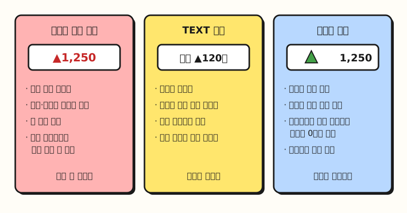 Even for the same change values, the right method depends on whether you'll reuse them in calculations, put them in a sentence, or view them by range (figure labels in Korean).
To sum up: if you want to keep using the numbers in your change column for calculations and just add ▲▼, use a custom format; if you're putting them into report sentences, use the TEXT function; and if you want to see ranges against a target like signals, icon sets are a good fit. For conditional formatting in general, see my post on Excel conditional formatting.
Notes
- Reference environment: The menu names and shortcuts in this post are based on Microsoft's help for Excel for Windows (Excel for Microsoft 365, Excel 2016 and later). Menu locations and shortcuts may differ in Excel for Mac.
- Excel for the web: Microsoft's help says you can't create custom formats in Excel for the web, but if you have the desktop app, you can open the file with Open in Excel and create them there.
- Limit: You can add between 200 and 250 custom number formats, depending on the language version of Excel you have installed.
- Regional settings: Depending on your computer's language and region settings, the formats shown by default in the Format Cells dialog, as well as the thousands separator and decimal symbol, may differ.
In the end, Excel increase/decrease indicators come down to a single principle of custom formats: "the value stays the same; only how it looks changes." If you remember the positive;negative;zero order, the quotation marks, and the square-bracket color rule, you can tweak the codes as your percentages or units change. I'm planning to add this format to my weekly report template and write it up again as I go. For more format symbols, see the guidelines for customizing a number format.
FAQ
- Do increase/decrease indicators turn numbers into text in Excel?
- Not if you added them with a custom format. Microsoft's help explains that a number format only changes how a value is displayed and doesn't affect the cell value used in calculations. However, results created with the TEXT function, or cells where you typed ▲ by hand, are text and are hard to use in calculations.
- How do I display negative numbers in red with an Excel custom format?
- Put the color name in square brackets at the very start of the second section (the negative section) of the format code. The English help example writes it like
[Blue]#,##0;[Red]#,##0. If the color name isn't accepted, choose a built-in format in the Number category that shows negative numbers in red, then move to Custom and copy the name written in the Type box. - What code adds arrows to percentage changes in Excel?
- If your percentage change is stored as a ratio like 0.125, use
[Red]"▲"0.0%;[Blue]"▼"0.0%;0.0%. The % multiplies the value by 100 and displays it with a percent sign, so 0.125 appears as ▲12.5%.
Related Posts
Posts that pair well with this one when you organize numbers and build reports in Excel.
- Excel conditional formatting: see numbers at a glance with colors, bars, and icons - Scanning changes with icon sets and color scales
- What is an Excel PivotTable? From definition to building and refreshing - PivotTable basics for summarizing numbers before you calculate changes
- Fixing #### in Excel: why cells show #### and how to fix it - When numbers don't show because of number formats and column width