Where is conditional formatting in Excel?

Select the cells, then click Conditional Formatting in the Styles group on the Home tab. In Excel for Windows, you can also apply rules like Data Bars, Color, and Icon Set right away from the Formatting tab of the Quick Analysis button (Ctrl+Q) that appears at the bottom right when you select data.

How do I color an entire row with conditional formatting?

Select the entire table range you want to color, choose "Use a formula to determine which cells to format" in New Rule, and enter a formula with $ only in front of the reference column. For example, select A2:F100 and enter the formula that checks whether D2 is less than 0, writing $D2 instead of D2, and every row with a negative value in column D will be colored.

Why isn't the color changing when I have multiple conditional formatting rules?

Rules are evaluated from top to bottom in the Conditional Formatting Rules Manager list, and when they conflict, only the higher rule is applied. New rules are added to the top by default, so check the order in Manage Rules and change it with Move Up or Move Down. It's also worth checking whether any rule has Stop If True turned on.

Can I hide the numbers and show only the bars in Excel data bars?

Yes. When you edit a Data Bars rule in Manage Rules, selecting "Show Bar Only" shows only the bar without displaying the cell value. Icon Sets have a "Show Icon Only" option that works the same way.

Excel Conditional Formatting: See Numbers as Colors, Bars, and Icons

Excel conditional formatting is a feature that lets you set rules so that colors, bars, or icons change automatically based on cell values. You can choose from Highlight Cells Rules that color only values above a threshold, Data Bars that show the size of a value as bar length, Color Scales that show highs and lows as color intensity, and Icon Sets that split values into ranges like traffic lights. Conditions the built-in rules can't handle can be defined yourself with a formula, and when there are multiple rules, the ones higher on the list are applied first.

"Isn't there a way to make the problem spots jump out of a table packed with numbers?" When you get an ad report or a sales table, all the numbers are there, but you often have to trace each row with your eyes to find where things actually dropped. If you color cells by hand, you have to recolor them every time the numbers change, and conditional formatting is a way to hand that job over to rules. In this post, I'll go over where to turn on Excel conditional formatting, how to choose rules, how to color entire rows with a formula, and how to sort things out when rules overlap, based on Microsoft's official help.

1. What Is Excel Conditional Formatting, and Where Do You Turn It On?

The help article introduces conditional formatting as a feature that makes patterns and trends in your data more apparent. You create rules that determine formatting based on cell values, and when the values change, the formatting follows those rules. You can apply it not only to cell ranges but also to Excel tables and PivotTable reports.

I found it easiest to understand as an automatic highlighter. Tell the highlighter in advance "make it yellow if it's under 100," and every time the number in a cell changes, Excel recolors it according to that rule.

There are two places to turn it on.

The ribbon: Select the cells you want to format, then click Conditional Formatting in the Styles group on the Home tab. From here you can choose Highlight Cells Rules, Top/Bottom Rules, Data Bars, Color Scales, Icon Sets, New Rule, Clear Rules, and Manage Rules.
Quick Analysis (Excel for Windows): When you select data, the Quick Analysis button appears at the bottom right of the selection, and you can also open it with Ctrl+Q. On the Formatting tab, hovering over an option previews the result. When numbers are selected, you get Data Bars, Color, Icon Set, Greater Than, and Top 10%; when only text is selected, you get Text Contains, Duplicate, Unique, and Equal To.

So which of these many rules should you choose?

2. Which Rule Should You Pick to Read Numbers at a Glance?

Choose based on whether you want to see "cells that crossed a threshold" or "differences in size between values."

Rule	Use it when	Official help description
Highlight Cells Rules	Finding values above or below a threshold, cells containing specific text, dates, or duplicate values	Greater Than, Between, Text that Contains, A Date Occurring, Duplicate Values, etc.
Top/Bottom Rules	Looking at the top 10, bottom 10%, or above/below average	The highest and lowest values in a cell range, and values compared to the average
Data Bars	Comparing the size of values by bar length	A longer bar is a higher value, a shorter bar a lower value
Color Scales	Viewing the distribution and highs/lows of values as color intensity	Two-color or three-color gradients; a three-color scale shows high, middle, and low values
Icon Sets	Marking values by dividing them into a few ranges	Three to five categories separated by threshold values, with each icon representing a range of values

Here's how that translates into situations that come up often at work.

Flag only targets that were missed: Select the conversions column, choose the comparison that colors cells less than a value under Highlight Cells Rules, and enter the threshold.
Compare costs by campaign: Apply Data Bars to the cost column, and you can see the big spenders by bar length before you even read the numbers. When you edit the rule, choosing Show Bar Only hides the numbers and leaves only the bars.
Scan percentage changes: Apply Color Scales to the change column, and high and low values separate by color.
Show status by range: With Icon Sets, you can divide ranges with traffic lights or arrows. When setting the conditions, choosing No Cell Icon for some ranges lets you leave warning icons only on cells that fell below the threshold.

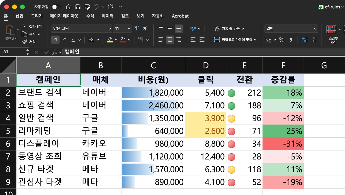Campaign table in Excel with conditional formatting: data bars on the cost column, icon sets on the conversions column, and color scales on the change column Actual Excel screen (sample data): data bars on cost, icon sets on conversions, color scales on change rate, and a Highlight Cells Rule coloring clicks under 4,000. (figure labels in Korean)

The help article also explains choosing Percentile as the type for the minimum and maximum values of Color Scales and Data Bars. This is because extreme values can keep the data from being displayed correctly. If your table has one or two unusually large sales, I recommend changing the minimum and maximum types to Percentile when editing the rule. But what about conditions that aren't on the built-in list, like "I want to color the entire row if column D is negative"?

3. When Built-In Rules Aren't Enough, How Do You Use a Conditional Formatting Formula?

In that case, open New Rule and choose Use a formula to determine which cells to format as the rule type. Then enter a formula in the Format values where this formula is true box. The formula must start with an equal sign (=) and must return a logical value of TRUE (1) or FALSE (0). Finally, click Format and choose the font, border, and fill to use when the condition is met.

The most confusing part here is cell references. According to the help article, if you click a cell on the worksheet to add it to the formula, an absolute reference (a fixed address like $B$2) is inserted, but if you want the reference to adjust automatically for each cell in the selected range, you need to use a relative reference. As shown in the table in the help article on reference types, $A1 is a mixed reference that locks the column and lets only the row move, so this form works well for coloring entire rows.

Coloring an entire row: Select A2:F100 and enter =$D2<0, and each row checks the column D value in its own row, coloring the whole row when it's negative. If you drop the $ and write =D2<0, the column shifts too, and each cell ends up looking at a different column.
Shading every other row: The help example =MOD(ROW(),2)=1 applies formatting only to odd rows, where the remainder of the row number divided by 2 is 1.
Flagging expiration dates: The help examples =B2<TODAY() finds dates earlier than today, and =B2<TODAY()+60 finds dates coming up within 60 days.
Finding duplicates: You can also use COUNTIF, as in =COUNTIF($A$2:$A$400,A2)>1, to color cells whose value appears two or more times.

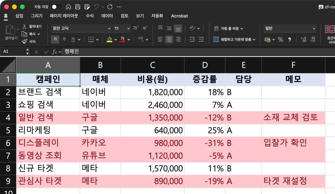Excel sheet where a conditional formatting formula colors entire rows whose change rate in column D is negative Actual Excel screen (sample data): with the =$D2<0 rule applied to A2:F9, only rows with a negative change rate in column D are colored from column A through F. (figure labels in Korean)

Once you start using formula rules, you end up with several rules on one range. Then which rule wins?

4. When There Are Multiple Rules, Which Is Applied First?

In the Conditional Formatting Rules Manager, which opens from Home > Conditional Formatting > Manage Rules, you can create, edit, delete, and see the order of rules. Rules are evaluated from top to bottom in this list, and a rule higher up takes precedence over the ones below it. The help article notes that new rules are added to the top of the list by default, so you should keep an eye on the order. You change the order with Move Up and Move Down.

When they don't conflict: If one rule makes text bold and another makes it red, both formats are applied.
When they conflict: If one rule changes the font to red and another to green, only the rule higher on the list is applied.
Stop If True: Checking this box stops evaluation at that rule. However, this check box isn't available for Data Bars, Color Scales, or Icon Sets rules.
When it overlaps with formatting you applied by hand: When a conditional formatting rule is true, it takes precedence over manual formatting in the same cell. If you delete the rule, the manual formatting remains.

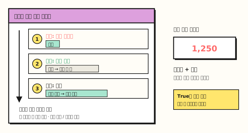How rules in the Conditional Formatting Rules Manager are evaluated from top to bottom, with only the higher rule applied when they conflict Example figure: the green rule that conflicts with the red rule above it is dropped, while the non-conflicting bold rule is applied as well. (figure labels in Korean)

Also, when you copy and paste cells with conditional formatting, use fill, or use Format Painter, new rules are created in the target cells. If you copy a table many times, similar rules can pile up in the Rules Manager, so it's a good idea to open the list now and then and clean it up.

※ Note: What If the Formatting Doesn't Show, or You Want to Remove It?

Cells with errors: Conditional formatting isn't applied to cells where the formula returns an error. The help article suggests using IS functions or the IFERROR function to return a value like 0 or "N/A" instead of the error.
Blank cells: A blank cell in the blank-cell rule is a cell with no data, and a cell with even a single space is considered text and treated differently from a blank cell.
PivotTables: You can't apply formatting based on unique or duplicate values to fields in the Values area; you can only format based on numbers.
Clearing rules: To clear only the selected cells, go to Conditional Formatting > Clear Rules > Clear Rules from Selected Cells; for the whole sheet, choose Clear Rules from Entire Sheet in the same menu. To delete just one specific rule, pick it in the Rules Manager.

To sum up, you can remember Excel conditional formatting in four groups: highlight rules that find cells crossing a threshold, Data Bars and Color Scales that compare size, Icon Sets that divide ranges, and formula rules for when none of those work. Just knowing that the rule higher on the list wins when rules overlap should cut down a lot on "why isn't the color changing?" moments. I'm going to try adding rules to my reports one by one and put this together again, so please refer to the official help for detailed settings for each option.

FAQ

Where is conditional formatting in Excel?: Select the cells, then click Conditional Formatting in the Styles group on the Home tab. In Excel for Windows, you can also apply rules like Data Bars, Color, and Icon Set right away from the Formatting tab of the Quick Analysis button (Ctrl+Q) that appears at the bottom right when you select data.
How do I color an entire row with conditional formatting?: Select the entire table range you want to color, choose "Use a formula to determine which cells to format" in New Rule, and enter a formula with $ only in front of the reference column. For example, select A2:F100 and enter the formula that checks whether D2 is less than 0, writing $D2 instead of D2, and every row with a negative value in column D will be colored.
Why isn't the color changing when I have multiple conditional formatting rules?: Rules are evaluated from top to bottom in the Conditional Formatting Rules Manager list, and when they conflict, only the higher rule is applied. New rules are added to the top by default, so check the order in Manage Rules and change it with Move Up or Move Down. It's also worth checking whether any rule has Stop If True turned on.
Can I hide the numbers and show only the bars in Excel data bars?: Yes. When you edit a Data Bars rule in Manage Rules, selecting "Show Bar Only" shows only the bar without displaying the cell value. Icon Sets have a "Show Icon Only" option that works the same way.

Here are posts worth reading together when organizing and reading numbers in Excel.

What Is an Excel PivotTable, and When Should You Use It? - PivotTable basics, where you can apply conditional formatting to summary tables too
Building PivotTable Reports With Slicers and PivotCharts - How to present summarized numbers with buttons and charts
VLOOKUP vs XLOOKUP: Which Excel Lookup Function to Use - Lookup functions that pull values from other sheets to complete a table