An Excel PivotTable is a feature that instantly summarizes totals, counts, and averages once you tell it "what to view the data by." Just drag a field into place and the table rebuilds itself, so you can quickly make reports like monthly sales or performance by channel without writing any functions. In this post, I go through what a PivotTable is, how to create one, practical examples, and the refresh you must do after changing the source data.
Why Use a PivotTable?
People often say, "To be good at Excel, you need to know how to use PivotTables." So today, let's look at what a PivotTable is, when to use it, and how to use it a bit more comfortably.
First, the dictionary meaning of "pivot" is a central point or axis of rotation, and you can think of Excel's PivotTable in terms of an axis too.

A PivotTable can be seen as a feature that takes the axis, or perspective, you want to look at and turns it into a table. Let me show you why PivotTables are great with the example below.
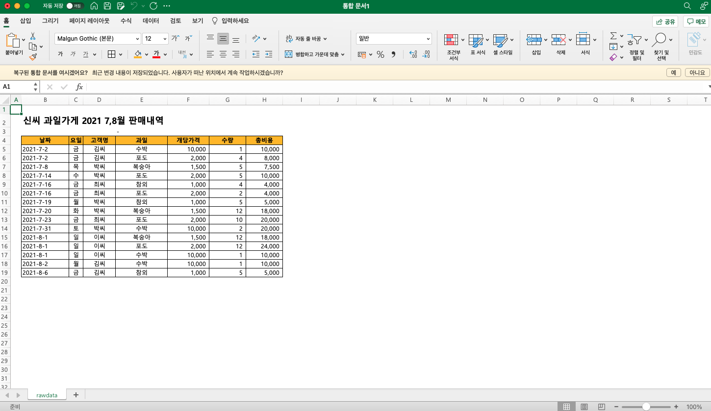
For example, if we have sales records for a certain period, we may want to analyze them from various perspectives to understand what drives purchases: which customers visited our store most, which items sold best, and so on. A PivotTable is exactly what lets you check data from many perspectives like that. Before I knew about PivotTables, I used to rebuild tables with functions every time I wanted a different view, but since a PivotTable lets you switch views instantly, there's no need to write complex formulas or start over whenever the criteria change.
How to Create a PivotTable in Excel
Step 1: Select the data and insert a PivotTable
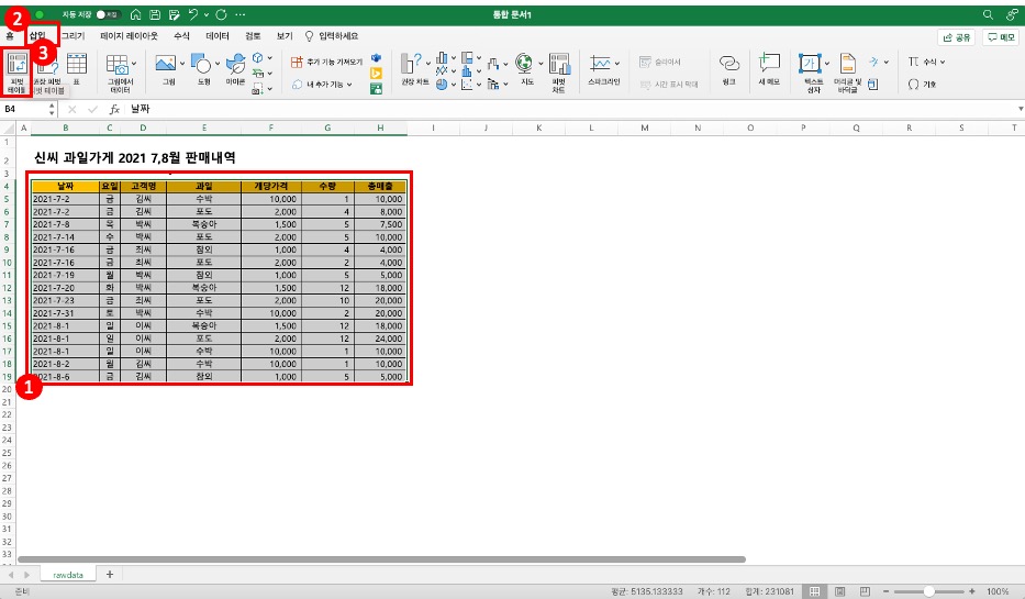
Select the data range you want to view in the PivotTable, then choose [Insert] > PivotTable.
Step 2: Set the range and location
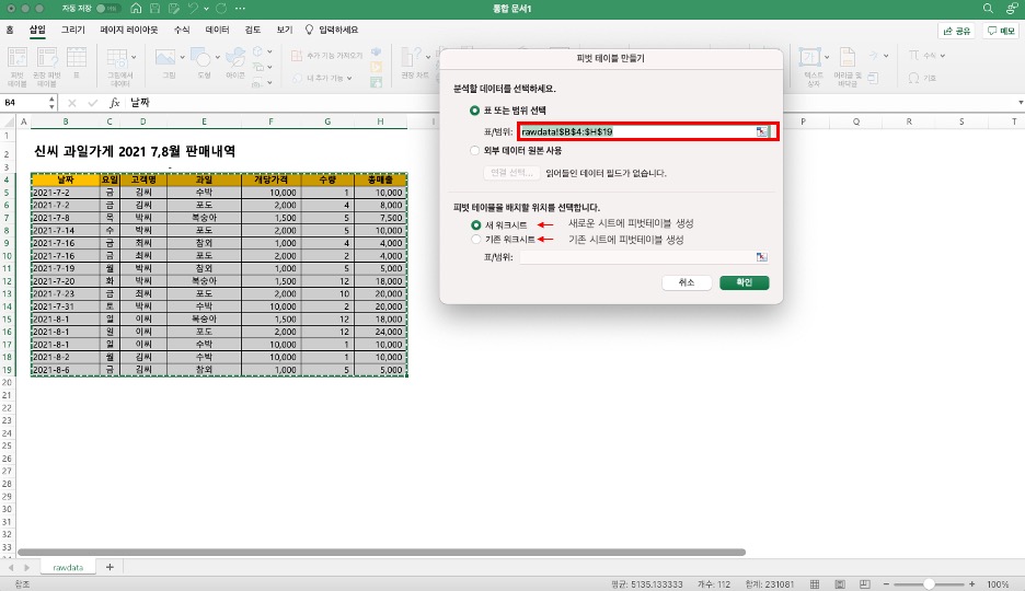
When the pop-up appears, double-check the data range, and choose whether to add the PivotTable to a new worksheet or an existing one.
Step 3: Set Rows and Values
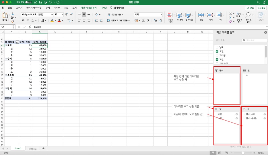
Put the criterion you want to view by in the "Rows" area, and the items you want to see for each criterion in the "Values" area.
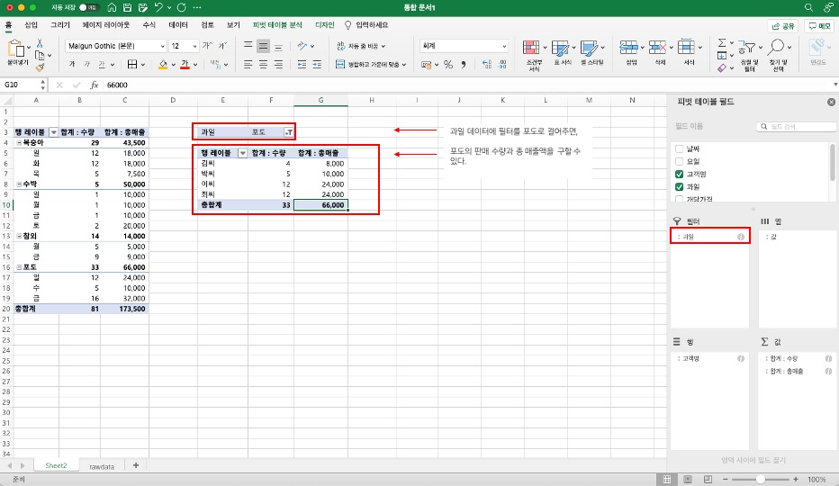
If grapes sold the most among the fruits and you want to see only grape data, you can use the filter feature. Put the fruit field in Filters and filter for grapes only, and you can see which customers bought grapes, plus each customer's grape quantity and total sales.
Step 4: Change the calculation function
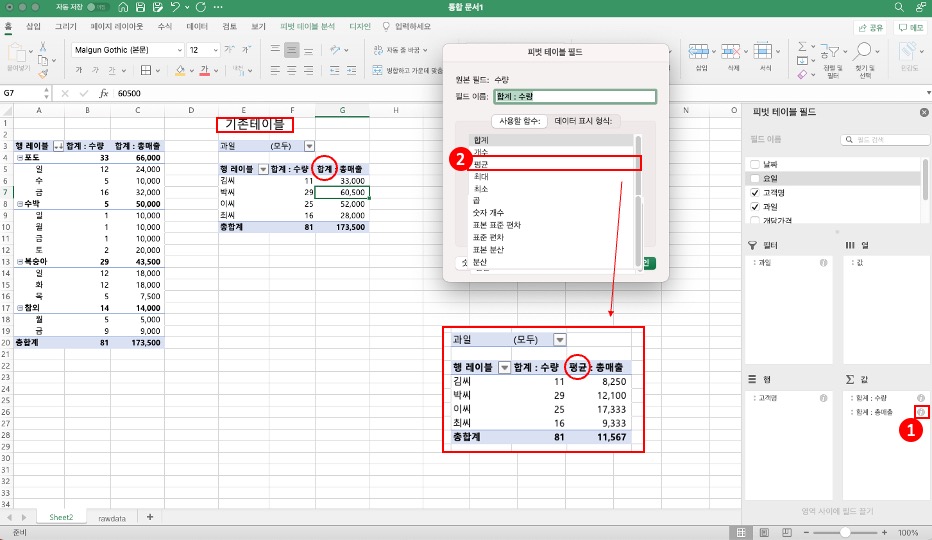
Values show up as a count or sum by default, but depending on the situation you may need an average, maximum/minimum, and so on. In that case, click the (i) button next to the value field to open a pop-up, where you can change the function.
There's also a way to calculate the items in a pivot with your own formulas, which I'll cover in my next post.
Practical PivotTable Examples
You may get the concept but still not have a feel for how it's used at work, so I've put together a few real-world use cases.
Analyzing monthly/quarterly sales trends
This is the most common use. If you have sales records with dates, put the date in Rows and use the Group feature to bundle them by month or quarter. For example, even if a year's worth of daily sales data takes up 365 rows, one grouping neatly organizes it into 12 months. Add "Product Category" to Columns, and you instantly get a month × category sales matrix. Because data scattered across days now shows up as a trend at a glance, you can quickly answer questions like "Why did sales drop this quarter?"

Comparing performance by category / owner
Put category or owner in Rows and sales or counts in Values, and a performance comparison table is done. I used this a lot at work to compare performance across ad channels: put channel names in Rows and impressions, clicks, and conversions in Values at the same time, and a channel performance comparison comes out without a single formula. Add Columns, and you can instantly build month × owner or channel × period matrices too. When I remember the days of building report tables by setting conditions one by one with SUMIFS, I really appreciate PivotTables.
Customer segment analysis
PivotTables are also handy when you want to classify customers by purchase frequency or spending range. For example, put purchase amount in Rows and use grouping to split it into ranges like "₩0–50K, ₩50K–100K, ₩100K and up," and you can see the number of customers and share of sales for each range at a glance. Change the value field's display format to a percentage, and you can immediately see each segment's share of total sales. This kind of analysis is really useful when planning a VIP customer management strategy.
Tips for Using PivotTables Better
Use date grouping
When you put a date field in Rows, it shows up by day by default, which means so much data that trends are hard to see. Right-click any date cell and choose "Group" to bundle by month, quarter, or year. Here's a tip! When grouping, select both "Months" and "Years" to get a clean year × month layout. If you select only "Months," data from the same month in different years gets merged together, so be careful.

Make it interactive with slicers
Choose "Insert Slicer" from the PivotTable menu to create button-style filters. Compared with drop-down filters, they're much more visually intuitive, and you can see at a glance which items are currently selected. Even better, one slicer can be connected to multiple PivotTables at once: place a sales PivotTable and an order-count PivotTable side by side, click a category on the slicer, and both are filtered at the same time, so you can build a pretty convincing dashboard with Excel alone. I've written up the steps for inserting slicers and connecting them to multiple PivotTables separately in my post on building PivotTable reports.

Link a PivotChart
Insert a "PivotChart" while the PivotTable is selected, and you get a chart linked to the PivotTable. What sets it apart from a regular chart is that when you change the PivotTable's filters or row/column layout, the chart updates automatically. When a report needs charts, you don't have to select a separate data range and build a chart; a few clicks and it's done. And when data is added, a refresh updates the chart too, so maintenance is easy.
Things to Watch Out for with PivotTables
PivotTables are convenient, but they won't work properly if the source data isn't clean. Keep a few things in mind.
- No blank rows or columns. If there's a blank row in the middle of your data, the PivotTable may decide the data ends there.
- Headers are required. Each column needs a name (header) in the first row to be recognized as a PivotTable field. If the data starts without headers, you end up with odd field names.
- Keep data types consistent. If numbers and text are mixed in the same column, sums and averages won't calculate correctly. Cells that look like numbers but are stored as text are a particularly common problem, so watch out.
- Refresh after changing data. If you edit the source data, you need to right-click the PivotTable → "Refresh" for the changes to show. Remember that it doesn't update automatically.
How to refresh a PivotTable
According to Microsoft's help article on refreshing PivotTable data, in Excel for Windows you can click Refresh on the PivotTable Analyze tab or press Alt+F5. To update all PivotTables in the workbook at once, choose Refresh All.
If you want the latest data every time you open the file, check "Refresh data when opening the file" on the Data tab of the PivotTable Options. The same help article also introduces an automatic refresh feature, but it says the feature is currently available to Microsoft 365 Insiders, so most people will need to click refresh themselves.
FAQ
- Why isn't any data showing up in my PivotTable?
- The most common causes are blank rows in the source data or missing headers. Check that the data range is selected correctly and that there are no blank rows in the middle. Also, after editing the source data, you need to right-click the PivotTable → Refresh for the changes to appear.
- How do I group dates by month in a PivotTable?
- Put the date field in Rows, then right-click any date cell and choose "Group." You can select the unit you want, such as months, quarters, or years. Note that grouping won't work if the dates are stored as text, so first check that the cell format is "Date."
- PivotTable vs SUMIFS: which should I use?
- If you only need one or two conditions on fixed criteria, SUMIFS is simpler. But if you need to explore data from multiple perspectives while frequently changing the criteria, a PivotTable is far more efficient. Because you can change criteria instantly with drag and drop, PivotTables are well suited to exploratory analysis.
- Can I reference PivotTable results from another sheet?
- The GETPIVOTDATA function lets you reference PivotTable values from other cells. If you build a formula by clicking a PivotTable cell, this function is entered automatically. However, the reference can break if the PivotTable's structure changes, so be careful.
Related Posts
Excel features that work well with PivotTables.
- Building PivotTable Reports | See It All with Slicers and PivotCharts - The next step: building reports with slicers and PivotCharts
- Excel Conditional Formatting | Seeing Numbers as Colors, Bars, and Icons - How to add colors and data bars to summarized numbers
- VLOOKUP vs XLOOKUP | Which Excel Lookup Function to Use When - Functions for pulling in values from other tables before building a PivotTable
- Removing and Finding Duplicates in Excel - How to clean up duplicates in the source data first
- How to Fix Garbled Korean Text in Excel Data - When Korean text breaks in a downloaded CSV