Excel formula errors come with different names, like #N/A, #VALUE!, #REF!, #NAME? and #DIV/0!, and each name is a clue that tells you what went wrong.
#N/A means the value you're looking for isn't there, and #REF! means a cell the formula pointed to is gone, so the name alone tells you where to start looking.
You can hide them all at once with IFERROR, but hiding errors without knowing the cause can leave wrong numbers in your report, so the safe order is fix first, then hide only what's left.
"My report was fine yesterday, and now it's full of #N/A."
If you've ever pasted data downloaded from an ad platform and pulled in revenue with VLOOKUP, you've probably seen this at least once.
So what should you check first for each error, and when is it fine to use IFERROR? In this post, I'll go through the causes and fixes for the five Excel formula errors you'll run into most, along with how to choose an error-handling function.
1. What does each Excel formula error tell you?
Microsoft's help on detecting formula errors describes the error values that appear in cells like this.
| Error value | Meaning |
|---|---|
| #DIV/0! | You divided by zero or a blank cell |
| #N/A | A function or formula can't find a value |
| #NAME? | Excel can't recognize text in the formula, such as a function name or range name |
| #NULL! | You used the intersection operator (a space) on two ranges that don't intersect |
| #NUM! | A function or formula contains an invalid numeric value |
| #REF! | A cell reference isn't valid (it was deleted or pasted over) |
| #VALUE! | The formula mixes different data types |
Error values are a lot like the warning lights on a car's dashboard. Just as the engine light and the tire light point to different problems, #N/A and #REF! point to different places too.
Putting tape over a warning light doesn't fix the car, and covering errors with IFERROR works the same way, so the first step is reading which warning light is on.
By the way, a cell filled with #### is different from the errors above. It's a display issue that happens when a column is too narrow or a date or time value is negative, and I covered it separately in my Excel #### fix post.
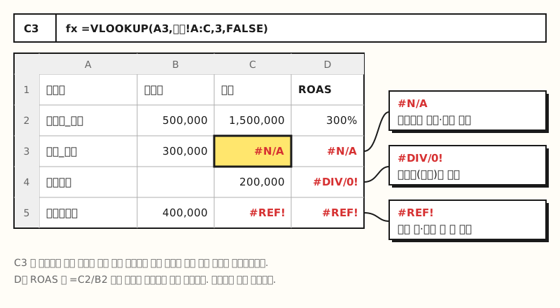 Example figure: a sample sheet made with made-up data, not an actual screenshot. Each error name points to a different place to check. (figure labels in Korean)
So how do you fix the five you'll see most often at work?
2. How do you fix the five most common Excel formula errors?
#N/A: when the value can't be found According to Microsoft's #N/A error help, this error shows up most often in XLOOKUP, VLOOKUP, HLOOKUP, LOOKUP and MATCH. First check whether the value really exists in your source data, and if it does, check these three things.
- Data type: If one side is stored as a number and the other as text, the lookup won't match even when the values look the same. For this case, see my post on converting numbers stored as text.
- Leading and trailing spaces: The help suggests using the TRIM function to remove them.
- Exact match: Set VLOOKUP's last argument, range_lookup, to FALSE, and set MATCH's match_type to 0. With an approximate match, you may get not only
#N/Abut also wrong values.
#VALUE!: when text gets mixed in where numbers should be
Microsoft's #VALUE! error help names calculating cells that contain hidden spaces or text with operators like + or * as a typical cause. Using a function, such as =SUM(A2:C2) instead of =A2+B2+C2, often solves it, and you can also add ISTEXT in a separate column to find the cells that return TRUE and re-enter them. The help also points out that dates aligned to the left are likely dates entered as text.
#REF!: when a referenced cell disappears
The example in Microsoft's #REF! error help makes it easy to understand. If you delete column C from =SUM(B2,C2,D2), the formula becomes =SUM(B2,#REF!,C2). If you notice right away, just undo with Ctrl+Z, and if you write it as a range like =SUM(B2:D2) from the start, Excel adjusts the formula on its own even when you delete a column in the middle. You'll also get #REF! when you ask for the 5th column of a 4-column range, as in =VLOOKUP(A8,A2:D5,5,FALSE).
#NAME?: when Excel can't read text in the formula
Microsoft's #NAME? error help names a typo in the function name as the top cause. Other causes include using a name that isn't defined, text that isn't wrapped in double quotes, a missing colon in something like B2:B12, and a function that can't be used because its add-in is turned off. Instead of typing function names by hand, picking them from the Formula AutoComplete list that appears as you type helps cut down on typos.
#DIV/0!: when you divide by zero or a blank cell
According to Microsoft's #DIV/0! error help, it happens when the divisor is zero or empty. If the cell just hasn't received data yet, you can make the formula calculate only when there's a divisor, as in =IF(A3,A2/A3,0).
For all five, fixing the cause comes first. So how should you handle the errors that still remain?
3. IFERROR, IFNA or XLOOKUP: what should you use to handle errors?
There are three main ways to show something else in place of an error.
| Method | Errors it catches | Good for | Watch out for |
|---|---|---|---|
| IFERROR(value, value_if_error) | #N/A, #VALUE!, #REF!, #DIV/0!, #NUM!, #NAME?, #NULL! | Replacing errors that remain after you've checked the cause, all at once | It hides every error, including typos and deleted references |
| IFNA(value, value_if_na) | #N/A only | Replacing only "not found" lookup results while keeping other errors visible | Other errors stay as they are |
| XLOOKUP's if_not_found | When no match is found | Lookup formulas that use XLOOKUP | If you leave it out, you get #N/A |
The errors handled by IFERROR, according to Microsoft's IFERROR function help, are the seven in the table above, and Microsoft's IFNA function help explains that IFNA returns the value you specify only when the formula returns #N/A. According to Microsoft's XLOOKUP function help, if you leave if_not_found empty, you get #N/A when there's no match.
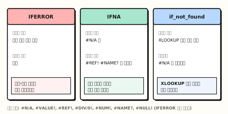 IFNA replaces only #N/A and leaves the other errors visible. (figure labels in Korean)
Here's how I choose.
- For lookup formulas, IFNA or if_not_found: This lets you turn only "campaigns not on the list" into "no match" while leaving a
#REF!caused by a wrong range visible. - For division, check the divisor with IF: It handles only the cases where the divisor is empty, so it doesn't cover up other mistakes.
- IFERROR last: The #DIV/0! help also warns that IFERROR and
IF(ISERROR())hide all errors, not just #DIV/0!, so you should first confirm that the formula works properly. The #NAME? help likewise recommends fixing the syntax instead of masking the error with IFERROR.
There's also a way to change only what's displayed while leaving the cell value alone. According to Microsoft's help on hiding error values, you can go to Home > Conditional Formatting > Manage Rules > New Rule, choose "Format only cells that contain", select "Errors" and change the font to white, and for PivotTables you can go to PivotTable Analyze > Options, open the Layout & Format tab and select "For error values show" to set the text shown instead. Keep in mind, though, that conditional formatting only changes the font color, so the value in the cell is still an error.
4. If errors show up in your weekly ad report, what order should you fix them in?
Let's say you're building a weekly report that pulls revenue from an Orders sheet into a campaign ad spend sheet with VLOOKUP, and calculates ROAS as revenue/ad spend. The data is just an example.
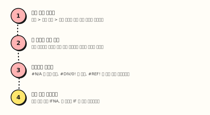 Hiding errors happens only in the last step. (figure labels in Korean)
- Collect where the errors are. Click Formulas > Formula Auditing > Error Checking, and Excel finds the cells with errors one by one.
- Break the formula down step by step. Open Evaluate Formula in the same group and click Evaluate, and the underlined part is calculated in turn, so you can see which piece produces the error. Microsoft's help on detecting formula errors places this feature under Excel for Windows, but the "Applies To" list of Microsoft's help on evaluating a nested formula one step at a time also includes Excel 2024 and 2021 for Mac, so depending on your version the menu may not appear.
- Fix by cause. For
#N/Ain the revenue column, start with trailing spaces in campaign names or number vs. text format differences. For#DIV/0!in the ROAS column, start with rows where ad spend is blank. For#REF!, start by checking whether a column was deleted last week. - Handle only what's left. For campaigns that truly had no orders this week, return 0 with something like
=IFNA(VLOOKUP(A2,Orders!A:C,3,FALSE),0), and for rows with no ad spend yet, leave a blank with something like=IF(B2,C2/B2,"").
Revenue   =IFNA(VLOOKUP(A2,Orders!A:C,3,FALSE),0)
ROAS      =IF(B2,C2/B2,"")
Set up this way, if the sheet range shifts next week and a #REF! appears, IFNA won't cover it up, so you'll spot it right away. If metric formulas like ROAS are confusing, my post on calculating ad performance metrics may help too.
5. Does the same approach work in Google Sheets?
Google Sheets uses error values with the same names. Google's ERROR.TYPE help shows that this function returns the error type as a number: 1 through 7 are #NULL!, #DIV/0!, #VALUE!, #REF!, #NAME?, #NUM! and #N/A in that order, and all other errors are 8. In a sheet with lots of errors, putting =ERROR.TYPE(A3) in the next column and grouping them by type with a filter makes it easier to decide where to start.
That said, a few functions behave slightly differently from Excel.
- IFERROR's second argument: In Google's IFERROR help, the second argument is optional, and if you leave it out you get a blank instead of the error. Microsoft's IFERROR help lists both arguments as required.
- IFNA: Google's IFNA help also lists both arguments as required, and it returns the specified value only for
#N/A.
※ For reference, the setting that turns off Excel's error indicator triangles is under Error Checking in File > Options > Formulas. In English it's labeled "Enable background error checking", but the Korean versions of the two help pages label this checkbox differently, so the name may vary by version or language. Turning it off makes errors harder to spot, so I recommend leaving it on unless the file is meant for sharing.
Wrapping up
Since the name of an Excel formula error is a clue to its cause, most of them get solved by checking the lookup value and format for #N/A, the deleted reference for #REF!, and the divisor for #DIV/0! first. If you get into the habit of handling only the errors left after fixing the cause, narrowly with IFNA or IF, and using IFERROR only when you know what it's hiding, you can trust the numbers in your reports. If I come across new error cases while building reports, I'll share them here. For how to choose a lookup function in the first place, check out my VLOOKUP vs XLOOKUP post.
FAQ
- How do I get rid of the #N/A error in Excel?
- First check that the lookup value exists in the source data, that the number and text formats match, and that there are no leading or trailing spaces. For VLOOKUP, set the last argument to FALSE so it looks for an exact match. If the value truly doesn't exist, you can show something like 0 or "none" instead with the IFNA function or XLOOKUP's if_not_found argument.
- What's the difference between IFERROR and IFNA?
- IFERROR replaces all of #N/A, #VALUE!, #REF!, #DIV/0!, #NUM!, #NAME? and #NULL! with the value you specify, while IFNA replaces only #N/A. If you use IFNA in lookup formulas, only "value not found" is handled, and other problems like range errors or typos in function names stay as errors so you notice them right away.
- Can I find all cells with Excel formula errors at once?
- Click Error Checking in the Formula Auditing group on the Formulas tab, and Excel finds the cells with errors one after another. With Evaluate Formula in the same group, you can calculate the selected cell's formula one step at a time to see where the error comes from. Depending on your Excel version, though, the Evaluate Formula menu may not be available.
More related posts
Here are some posts worth reading alongside this one when you work with Excel formulas and data.
- VLOOKUP vs XLOOKUP: Which Excel Lookup Function to Use - How to choose the lookup functions where #N/A shows up most often
- Excel #### Error Fix: Why Cells Show #### and How to Fix It - How to fix the #### display that's easy to confuse with formula errors
- Excel PivotTable Guide: What It Is, How to Create and Refresh - How to summarize your cleaned-up data with a pivot table