A common reason Excel doesn't recognize numbers is that the numbers are stored as text.
They look like numbers, but Excel treats them as text, so they get left out of totals, sorting gets jumbled, and VLOOKUP can return #N/A.
You can spot them by the green triangle in the top-left corner of the cell, and turn them into real numbers with the Convert to Number menu, Paste Special's Multiply, or the VALUE function.
"I added up the revenue column with SUM, but the total is oddly small." If you've moved data downloaded from an ad platform or an online store's admin into Excel, you've probably run into this at least once. The numbers are clearly visible, yet they aren't counted in the calculation, which is frustrating. Working in digital marketing, I often have to clean up downloaded reports in Excel, so I wanted to properly sort out this problem once. In this post, following Microsoft's help article on converting numbers stored as text, I'll go over the cause, how to spot it, three ways to convert, and what to check when it doesn't convert.
1. Why Doesn't Excel Recognize Numbers as Numbers?
The help article on fixing text-formatted numbers gives two typical cases where numbers end up stored as text.
- When you type into a text-formatted cell: If you enter a number in a cell formatted as text, it's stored as text, not as a number.
- When you import or copy from outside: This is when data is imported or copied as text from a database or another external data source.
Given that Excel's error-checking rule is named "Numbers formatted as text or preceded by an apostrophe," numbers entered with an apostrophe (') in front are also flagged by the same warning. To put it another way, it's like sticking number stickers on calculator buttons. You see a 7, but pressing it doesn't calculate anything. So how can you tell whether the numbers in your sheet are these "sticker numbers"?
2. How Do You Spot Numbers Stored as Text?
The help article points to two signs. Numbers formatted as text are aligned to the left instead of the right in the cell, and a small green triangle (error indicator) often appears in the top-left corner of the cell. Left this way, they can cause problems in calculations or mix up the sort order. According to the SUM function help, SUM ignores text values and adds only numeric values, so the total can come out smaller than you expect.
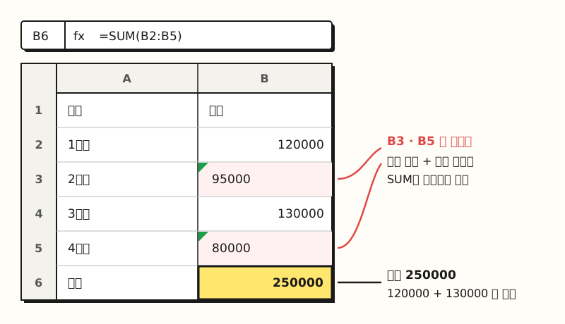 Example figure: cells B3 and B5, aligned to the left, are text, so they aren't included in the
=SUM(B2:B5) total (sample data). (figure labels in Korean)
It's also a problem for lookup functions. The help article on fixing the #N/A error explains that if VLOOKUP is set to look up a number but the source data is stored as text, the data types don't match and you can get #N/A.
When you're matching two sheets by product code or order number and it can't find a value that's clearly there, start by suspecting that one side is text.
3. How Do You Convert Numbers Stored as Text to Numbers in Excel?
Grouping the methods in the help article by situation gives three.
| Method | Use it when | Steps (Microsoft help wording) |
|---|---|---|
| Convert to Number | You can see the green triangle | Select the cell, select the error indicator at the top left (or Alt+Shift+F10), then choose Convert to Number from the menu |
| Paste Special Multiply | You want to convert everything at once without green triangles | Type 1 in a blank cell and copy it, then on the range to convert use Paste Special > Multiply under Operation |
| VALUE function | You want to keep the original and convert in a new column | Fill the next column with something like =VALUE(E23), then copy the results and use Paste Values |
Convert to Number is the simplest method. Select the cell or range with the green triangle, a warning button appears next to it, and you click Convert to Number. If you want to keep the values as they are and just remove the warning, choose Ignore Error. If you don't see the triangle at all, error checking may be turned off. You can turn it back on by selecting Enable background error checking under File > Options > Formulas.
Paste Special Multiply converts text to numbers by multiplying each cell by 1. Since it's multiplied by 1, the visible value stays the same, but the actual cell content becomes a number. The steps are shown in the figure below.
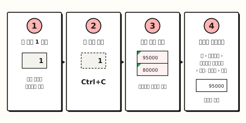 Multiplying by 1 leaves the value unchanged, so only the content becomes a number. After converting, delete the cell where you typed 1. (figure labels in Korean)
The VALUE function converts text that represents a number into a number. Insert a new column next to the text column, put the cell inside the parentheses of =VALUE() and fill down, then copy the results and paste them over the first cell of the original column using the arrow under Paste on the Home tab > Paste Special > Paste Values (Ctrl+Shift+V).
For reference, the VALUE function help notes that you generally don't need VALUE in formulas, because Excel automatically converts text to numbers as needed, and that the function is provided for compatibility with other spreadsheet programs. That's why I introduced it in this post only for cleaning up an entire column.
But if some cells still won't turn into numbers even after this, what should you check?
4. What Should You Check When Convert to Number Doesn't Work?
The most common cause is invisible spaces or characters. The top ten ways to clean your data help article explains that data imported from external sources can contain leading or trailing spaces or nonprinting characters.
- TRIM function: Removes all spaces except single spaces between words. However, it's designed for the regular space character with value 32, so TRIM alone can't remove the nonbreaking space character with value 160, which is commonly used in web pages as
. - CLEAN function: Removes nonprinting characters (7-bit ASCII values 0 through 31).
- SUBSTITUTE function: Used alongside them to replace characters like value 160 with characters TRIM and CLEAN can handle.
For data where the decimal point and thousands separator differ by country, the NUMBERVALUE function is handy. It converts text to a number regardless of locale, and if you specify the separators yourself, as in =NUMBERVALUE("2.500,27",",","."), it returns 2,500.27. It also ignores spaces in the text, even in the middle, so " 3 000 " becomes 3000.
Data downloaded from accounting software sometimes has the minus sign on the right, like 156-. In that case, as in the help example, use =LEFT(A2,LEN(A2)-1)*-1 to drop the last character and multiply by -1 to get -156.
※ Note: Are There Numbers You Should Keep as Text?
Not every number needs to be converted to a number. The help article on formatting numbers as text explains that for identifiers you don't calculate with, keeping them as numbers can actually change the value.
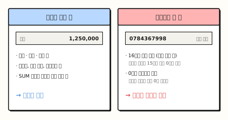 It's less confusing if you split them by whether a value is something you add up and average, or an ID you attach like a name tag. (figure labels in Korean)
Excel's numeric precision is up to 15 digits, so if you enter a number with 16 or more digits, like a card number, as a number, everything after the 15th digit turns into 0, which is why the help article recommends text format for these. Product codes that start with 0 also lose their leading zeros when entered as numbers, so you need to keep them as text or preserve the digit count with a custom number format like 0000000000.
So it's safer to keep values you add and compare, like amounts, quantities, and clicks, as numbers, and values you only attach, like order numbers or product codes, as text. However, for two sheets you'll match with VLOOKUP, you need to make the format of the code column the same on both sides.
The menu names in this post follow the help article for the versions the conversion article applies to: Excel for Microsoft 365 and Excel 2024, 2021, 2019, and 2016. For Excel for the web, the VALUE function steps are described a little differently.
To sum up, when Excel doesn't recognize numbers, it's often because they're stored as text. Check for the green triangle, then convert them with whichever fits your situation: Convert to Number, Paste Special Multiply, or the VALUE function. When a total looks off while I'm cleaning up a downloaded report, I try to check the alignment and the green triangle first. For more detailed steps, please refer to Microsoft's help article.
FAQ
- Why aren't my numbers included in the total in Excel?
- There's a good chance the numbers are stored as text. According to Microsoft's SUM function help, SUM ignores text values and adds only numeric values. If the cell is aligned to the left or has a green triangle in the top-left corner, select the cell and click Convert to Number from the warning button.
- How do I convert numbers stored as text if I don't see a green triangle?
- Turn on Enable background error checking under File > Options > Formulas and the green triangle will appear again. Alternatively, type 1 in a blank cell, copy it, and apply Paste Special > Multiply to the range you want to convert, or use the VALUE function in the next column.
- What do I do with cells that don't change even after clicking Convert to Number?
- They may contain leading or trailing spaces or nonprinting characters. Remove spaces with the TRIM function and nonprinting characters with the CLEAN function, and if data from a web page contains the nonbreaking space with value 160, replace it first with the SUBSTITUTE function.
Related Posts
Here are posts worth reading together when cleaning up downloaded data in Excel.
- How to Fix Broken Korean Text in Excel Data - Fixing garbled Korean text when opening a downloaded CSV in Excel
- What Is an Excel PivotTable? From Creating to Refreshing - How to summarize cleaned-up numeric data by multiple criteria
- VLOOKUP vs XLOOKUP: Which Excel Lookup Function to Use - Comparing lookup functions for matching two sheets by code