Masking data in Excel means leaving the original cells as they are and using a function in the next column to show part of a name, phone number or email with a symbol like * instead.
To replace characters at a fixed position, use the REPLACE function; to keep only a few characters at the start and end and fill in the middle, combine LEFT, RIGHT, LEN and REPT.
Keep in mind, though, that what a function hides is only the "displayed value," so masking isn't finished until you've also decided what to do with the original column before the file goes out.
"I need to announce the event winners, but how do I hide their names and phone numbers?" In marketing, there are moments when you need to show only part of someone's personal information, like announcing winners or sending a list to an outside partner. You can't rewrite hundreds of entries one cell at a time, so you want a function that handles it in one go. In this post I'll cover formulas for hiding part of personal data in Excel, and what you should check before sharing the file.
Does masking in Excel delete the original data?
Masking with functions doesn't edit the original. It reads the original and builds the masked result in a new column. If phone numbers are in column B, you put a formula in column C that shows the masked number. Doing it this way keeps the original intact, so you can rebuild the result if you make a mistake.
Think of it like a window envelope with a clear plastic window over the address. The whole letter is still inside, but from the outside you only see the part showing through the window. A masked column works the same way: only part of it shows on the surface, but if the original column is still in the same file, anyone who opens the envelope can see everything. I'll come back to this difference in the last section. First, let's look at which functions to use.
1. Which functions are used for masking in Excel?
Most masking formulas are a combination of the few functions below. All descriptions are based on Microsoft's official help articles.
| Function | What it does | Where it's used in masking |
|---|---|---|
| REPLACE(old_text, start_num, num_chars, new_text) | Replaces a set number of characters starting at a given position with other text | Fixed-position parts, like the middle four digits of a phone number |
| LEFT / RIGHT(text, [num_chars]) | Returns a set number of characters from the start or end of text | The characters you keep at the start and end |
| LEN(text) | Counts the characters in text (spaces count as characters) | Calculating how many characters to hide |
| REPT(text, number_times) | Repeats text a set number of times | Making multiple * to match the length |
| SEARCH(find_text, within_text) | Returns the position of the character you're looking for | Finding the position of @ in an email |
| & operator | Joins text together | Combining the pieces into one |
In the example from the REPLACE function help article, =REPLACE(A2,6,5,"*") replaces five characters starting at the sixth character of abcdefghijk with a single *, returning abcde*k.
The thing to notice here is that the number of characters you replace and the number you insert don't have to match.
So if you want to keep the original length after masking, you need to put as many * in new_text as the number of characters you're replacing.
According to the LEFT function and RIGHT function help articles, if you omit num_chars it's assumed to be 1, and if you enter a number larger than the text length, the whole text is returned. The REPT function help article explains that if the repeat count is 0, it returns empty text (""), and this behavior is exactly what causes trouble with two-character names in the next section.
2. How do you hide the middle character of a name with *?
If all the names have three characters, as most Korean names do, the simplest way is to replace the second character with REPLACE.
=REPLACE(A2,2,1,"*")
If A2 is 김하늘, you get 김*늘.
But a real list will have a mix of two-character and four-character names too.
That's why a common formula keeps only the first and last characters and hides the middle according to length, and in that case two-character names need separate handling.
=IF(LEN(A2)=2, LEFT(A2,1)&"*", LEFT(A2,1)&REPT("*",LEN(A2)-2)&RIGHT(A2,1))
If you use the second part of the formula as-is on a two-character name, LEN(A2)-2 becomes 0, REPT returns empty text, and 이준 comes out unchanged as 이준.
By using IF to split out the two-character case and replace only the last character with *, names are masked according to their length: 남궁민수 becomes 남**수 and 이준 becomes 이*.
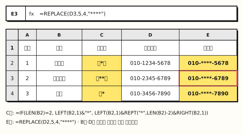 Example figure: names in column B and phone numbers in column D masked with formulas in columns C and E (sample data, not a real screenshot; figure labels in Korean).
3. How do you hide part of a phone number or email?
If phone numbers are all stored in the same format, hyphens included, like 010-1234-5678, the middle four digits always sit at a fixed position (four characters starting at the fifth), so a single REPLACE does the job.
=REPLACE(A2,5,4,"****")
The result is 010-****-5678.
However, if some numbers have no hyphens or have only three digits in the middle, the wrong part will get masked, so I recommend first putting =LEN(A2) in the next column to check that all the lengths are the same.
Showing only the last four digits is an approach Microsoft itself uses as an example in its help article Display only the last four digits of identification numbers.
The formula =CONCATENATE(REPT("****-",3), RIGHT(B3,4)) turns a card number into something like ****-****-****-5555.
According to the CONCAT function help article, CONCATENATE has been replaced by CONCAT but is still available for compatibility, and the & operator gives the same result, so you can also write =REPT("****-",3)&RIGHT(B3,4).
With email, the ID length varies, so you need to find the position of @ first. Here's a formula that keeps only the first two characters of the ID.
=LEFT(A2,2)&REPT("*",SEARCH("@",A2)-3)&MID(A2,SEARCH("@",A2),LEN(A2))
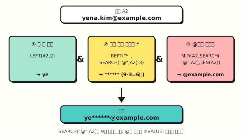 Example figure: how
yena.kim@example.com becomes ye******@example.com through the three pieces (sample address; figure labels in Korean).
As the SEARCH function help article explains, SEARCH returns the position of the character you're looking for, and returns a #VALUE! error if it can't find it.
Per the MID function help article, MID returns a set number of characters from a starting position, and if you ask for more than what's left, it only returns up to the end of the text, which is why LEN(A2) is used as a generous length.
This formula assumes addresses whose ID is at least three characters long, so if there are values missing @ or addresses with very short IDs mixed in, give the results a quick scan.
4. What should you check before sharing a masked file?
Going back to the window envelope analogy, sending a file with masked columns as-is is like handing over the letter, envelope and all. Microsoft's last-four-digits help article suggests hiding the column with the original data and protecting the worksheet so the original can't be viewed, but Microsoft's own Protect a worksheet help article clearly states that worksheet-level protection is not intended as a security feature. It explains that worksheet protection prevents people from editing locked cells, and that it's different from file protection, which uses a password to stop people from opening the file at all.
So when you send a file outside, it's safer to make a copy that contains only the masked values.
- Step 1: Copy the original workbook to make a copy. The help article on replacing formulas with their results also recommends making a copy of the workbook before you replace anything.
- Step 2: In the copy, select the masked columns, copy (Ctrl+C) and paste (Ctrl+V), then choose Values Only from the Paste Options. The formulas are permanently replaced with their results.
- Step 3: After confirming they've become values, delete the original columns. As the #REF! error help article explains, deleting cells that formulas refer to causes a #REF! error, so don't delete the originals before converting to values.
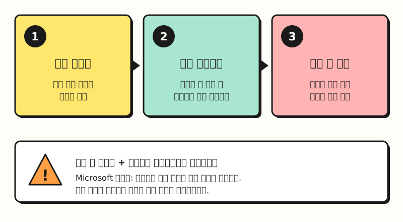 Example figure: instead of hiding columns and protecting the sheet, make a copy with only values and send that (figure labels in Korean).
The Protection and security in Excel help article says to always think twice before distributing workbooks that may contain sensitive personal information such as credit card numbers or resident registration numbers, and it also explains how to encrypt the file itself with a password. How much you need to hide should follow your company's personal data handling standards or the guidance of the responsible team first.
※ Notes: versions and data formats
- Supported versions: the REPLACE, LEN, REPT, MID and SEARCH help articles list Excel for Microsoft 365, Excel 2024, 2021, 2019 and 2016. The last-four-digits help article lists Excel for Microsoft 365 and Excel 2024 and 2021 (each including the Mac version).
- Functions ending in B: the help articles say REPLACEB, LEFTB, RIGHTB, MIDB, LENB and SEARCHB are no longer used, so use the versions without B, which count characters rather than bytes.
- Spaces: LEN counts a space as one character, so if a name has spaces before or after it, the number of asterisks in the middle will change. I covered how to find cells that look blank in my post on finding blank cells in Excel.
To sum up, masking in Excel is a set: hide fixed-position values with REPLACE, hide values of varying length with a LEFT, RIGHT, LEN and REPT combination, and when sharing, send a copy with only values. I plan to go back through these steps whenever I handle a list, so for the detailed behavior of each function, please refer to the official Microsoft help articles linked above.
FAQ
- How do I replace only the middle character of a name with an asterisk in Excel?
- If all the names have three characters, replace the second character with something like =REPLACE(A2,2,1,"*"). If two-character and four-character names are mixed in, it's safer to measure the length with LEN and use IF to split a formula that fills the space between the first and last characters with REPT. REPT returns empty text when the repeat count is 0, so two-character names need separate handling.
- What's the Excel formula for masking phone numbers?
- If the numbers all share the same format with hyphens, like 010-1234-5678, you can hide the middle four digits with =REPLACE(A2,5,4,"****"). If some numbers lack hyphens or have a different number of middle digits, the positions will be off, so check the length with LEN first.
- Is it safe to hide the original column and protect the sheet?
- Microsoft's Protect a worksheet help article explains that worksheet-level protection is not a security feature. It stops people from editing locked cells, so for a file going outside, it's safer to make a copy with the masked columns converted to values, delete the original columns, and then send it.
Related posts
Posts worth reading alongside this one when cleaning up Excel data.
- Find and Highlight Blank Cells in Excel: Go To Special, Conditional Formatting, ISBLANK - how to check for blank cells and cells with spaces before masking
- Find and Remove Duplicates in Excel: Remove Duplicates, Conditional Formatting, UNIQUE - how to clean up rows where the same person appears twice in a list
- What Is an Excel Pivot Table? From Creating to Refreshing - how to summarize a cleaned-up list by multiple criteria