To create a pivot table in Google Sheets, select data with headers, click Insert > Pivot table, and add rows, columns, and values in the panel that opens on the side. With the October 2026 update, there's now a compact form layout that stacks row fields in a single column with indentation, and compact-form pivot tables made in Excel can now be imported and exported with their layout intact. Another difference from Excel is that the pivot table refreshes on its own when you edit the source data.
"I used pivot tables all the time in Excel, but where do I make one in a shared sheet?" It's a question that comes up at least once after a team moves its shared ad report to Google Sheets. The menu names and panel layout are a little different from Excel, so it can feel unfamiliar at first. So in what order do you build one in Google Sheets, and what's different about the new compact layout? In this post, I'll cover the basic steps for creating a Google Sheets pivot table, the new layout, and what to know when exchanging files with Excel.
How do you create a pivot table in Google Sheets?
Here are the steps from the Create and use pivot tables Help article, for computer.
- Select your data: Select the source data cells you want to summarize. The Help article points out that each column needs a header, so if your table is just a run of numbers with no headers, add names to the first row first.
- Insert > Pivot table: Click it in the top menu, and if the pivot table sheet doesn't open, click on that sheet.
- Add rows and columns: In the panel that opens on the side, click Add next to "Rows" or "Columns" and choose the fields to group by. For example, you might put channel and campaign in rows.
- Add values: Click Add next to "Values" and choose the fields to calculate, like cost or clicks, and change how they're summarized, such as sum or count, using the down arrow next to the item.
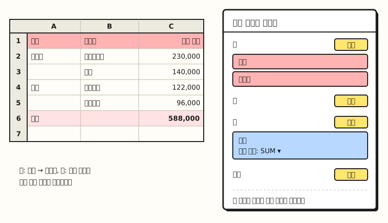 Example: a diagram, not an actual screenshot. With sample data, the fields placed in the Rows and Values areas of the right panel determine the shape of the table on the left (figure labels in Korean)
When you select data, Sheets sometimes shows suggested pivot tables first. According to the Help article, high-confidence suggestions may even be inserted automatically when you create one. If that's a hassle, go to Tools > Suggestion controls and turn off "Enable pivot table suggestions." Once the table is created, it's time to polish it into a report.
What other settings help when using it as a report?
The Customize a pivot table Help article covers features for polishing the table. For tables you view in the same format every time, like a weekly ad report, I recommend learning these four first.
- Sorting and totals: Under "Order" and "Sort by" in "Rows" or "Columns," sort alphabetically or by value, and check Show totals to show row and column totals.
- Viewing as percentages: Under "Show as" in "Values," click Default and choose a percentage option to see shares as ratios instead of amounts.
- Grouping: Right-click a cell in date format and choose Create pivot date group to group by date unit, and for numbers, use Create pivot group rule to split them into ranges.
- Filters: Click Add next to "Filters" to filter by condition (is not empty, text contains, etc.) or uncheck items to hide by value.
With the editor panel open, you can also rename row and column headers by clicking them, but the Help article notes that "Grand Total" can't be renamed.
How is it different from Excel pivot tables?
The basic idea of building a table by placing fields in four areas, rows, columns, values, and filters, is the same as an Excel PivotTable. But the difference you'll notice most is refreshing, and it's also good to know which Excel features work similarly in Sheets.
- Refreshing: The Help article says Google Sheets pivot tables refresh automatically when the source data cells change. In Excel, according to the refresh Help article, automatic refresh is still a feature available to Microsoft 365 Insiders, so outside the Insider program you have to refresh manually with Refresh on the PivotTable Analyze tab or Alt+F5.
- Viewing details (also in Excel): Double-clicking a value cell opens a new sheet with only the source rows that make up that number. When a total looks off, you can immediately see which rows were added.
- Calculated fields (also in Excel): Under Add > Calculated field next to "Values," you can create new values with SUM or a custom formula. Remember that field names with spaces need to be wrapped in quotes.
When several people edit the source in a shared sheet, not having to worry about forgetting to refresh is quite convenient. But there was one thing Excel users had been missing: the shape of the table.
How is the new compact layout different from outline form?
The Google Workspace Updates announcement distinguishes the two layouts like this.
- Outline form: Each row field takes up its own column. If you put channel and campaign in rows, channel goes in column A and campaign in column B.
- Compact form: All row fields are stacked in a single column, with indentation and expand/collapse buttons in place to show the hierarchy.
As an analogy, compact form is like a computer's folder tree. Just as subfolders inside a folder appear indented one step and you only click the arrow to expand them when needed, campaigns sit indented under each channel, and you can collapse and expand by channel. Even as you add three or four row fields, the table doesn't keep stretching sideways, so it can be easier to read on a narrow laptop screen or in report screenshots.
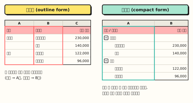 Example: sample data. Outline form on the left uses two columns for row fields, while compact form on the right stacks them in one column with indentation (figure labels in Korean)
According to the announcement, you can choose the layout right in the pivot table editor. However, at the time of writing, the Help article doesn't yet list the exact menu name for this option, so look for the layout-related item in the editor panel.
What changed when exchanging Excel files?
The part of this update that people who also use Excel will welcome most is importing and exporting. According to the announcement, until now compact-form pivot tables made in Excel turned into outline form when imported into Google Sheets, but now the original layout is preserved, and it stays that way when you export back to Excel.
This matters because of Excel's default. The Excel Help article on PivotTable layout describes compact form as the default layout form for PivotTables, which means that unless you've changed the default layout, PivotTables created in Excel are made in compact form. This may cut down on reworking tables whose shape changed after you uploaded Excel reports from clients or other teams to Sheets.
Besides compact and outline, Excel also has tabular form, which gives each field its own column, and you can switch layouts under Report Layout on the Design tab. This Google Sheets announcement only mentions compact and outline form, so it's worth checking separately how tabular form is handled.
※ Note: Can you use it right now?
The compact layout isn't opening to all accounts at once; it's rolling out in stages.
| Type | Rollout start | Notes |
|---|---|---|
| Rapid Release domains | October 22, 2026 | Gradual rollout, up to 15 days for the feature to appear |
| Scheduled Release domains | November 6, 2026 | Gradual rollout, up to 15 days for the feature to appear |
It's available to all Google Workspace customers and users with personal Google accounts, and there's no admin setting to turn it on or off. So even within the same company, some people may not see the option yet. Before sharing a sheet set to compact form, I recommend checking that it looks the same on the viewer's screen.
To sum up, you create a Google Sheets pivot table with Insert > Pivot table and add rows, columns, and values in the panel, and the biggest difference from Excel is that it refreshes on its own when the source changes. With the compact layout added, matching table shapes with Excel has become much easier. I'm planning to check again whether the layout stays intact when I move reports I receive in Excel into Sheets. For more detailed settings, please see the Customize a pivot table Help article.
FAQ
- Do I need to refresh Google Sheets pivot tables manually?
- According to Google's Help article, pivot tables refresh automatically whenever the source data cells change. You don't need to click a separate refresh button as in Excel.
- What's the difference between compact and outline pivot table layouts?
- Outline form uses one column per row field, while compact form stacks all row fields in one column and shows the hierarchy with indentation and expand/collapse buttons. Compact form has been rolling out gradually to Google Sheets since October 22, 2026.
- Does an Excel compact-form pivot table change shape when imported into Google Sheets?
- It used to turn into outline form, but according to the Google Workspace Updates announcement, the original layout is now preserved, including when you export back to Excel. Because of the staged rollout, timing may vary by account.
- Where is the button to create a pivot table in Google Sheets?
- Select the source data cells, then click Insert > Pivot table in the top menu. Each column needs a header, and you add fields by clicking Add next to Rows, Columns, and Values in the panel that opens on the side.
Related posts
Posts that pair well with learning pivot tables and sheet summaries.
- What is an Excel PivotTable, and when should you use it? - Pivot table basics and how to create one in Excel
- Building PivotTable reports | Slicers and PivotCharts - The next step in turning a pivot table into a report
- Google Sheets QUERY function basics - How to build a crosstab with one formula instead of menus