An Excel table turns an ordinary cell range into a single named block.
Once your data is a table, the range grows on its own when you add rows below it, and formulas use column names like Ads[Spend] instead of cell addresses like A2:A100.
That makes tables especially useful for sheets whose range keeps changing, such as an ad report that gets new data every week.
Have you ever asked, "Why isn't the SUMIFS I built last week adding up this week's data?" and then fixed each formula range by hand? Or refreshed a pivot table only to find the rows you just pasted were missing? In this post, let's look at how an Excel table differs from a regular range, how to create one, how to read structured reference formulas, and how to apply all of this to a weekly ad report.
How is an Excel table different from a regular range?
The Overview of Excel tables help article explains that you can convert a range of cells into a table to make it easier to manage and analyze a group of related data. On the surface it looks like striped formatting, but what really changes is how the range is handled. A table is made up of a header row, banded rows, calculated columns, a total row and a sizing handle, and the header row comes with sort and filter buttons by default.
Think of a regular range as a loose stack of paper on your desk, and a table as a labeled binder. With the loose stack, you have to point by position, like "from the third line on the left down to line forty," but with the binder you can just say "the Spend section of the Ads binder." Even if you slip in a few more pages, the binder's name stays the same, so formulas that use that name don't need fixing.
| Criteria | Regular range | Excel table |
|---|---|---|
| When you add rows | You must extend formula and pivot ranges yourself | Typing right below the table expands it |
| What formulas look like | =SUM(D2:D40) | =SUM(Ads[Spend]) |
| Filling a formula down a column | Drag the fill handle | Enter it in one cell and it applies to the whole column (calculated column) |
| Total row | Type SUM yourself | Turn on [Total Row] and pick a function from the drop-down |
| As a pivot source | You must reset the source range | Just refresh and added rows are included |
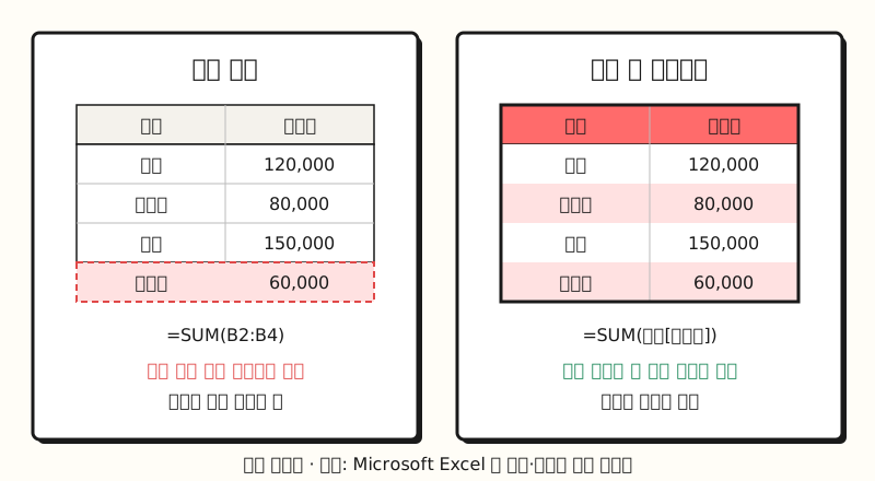 Add one more row to the same data: a regular range leaves the formula range as is, while a table widens along with it (figure labels in Korean).
So how do you create a table, and what should you change first once it's made?
1. How do I create an Excel table?
Here's the flow from the Create and format tables help article.
- Step 1: Select a cell or range in your data.
- Step 2: On the [Home] tab, select [Format as Table] and choose a style. As a shortcut, pressing Ctrl+T or Ctrl+L on Windows opens the [Create Table] dialog box.
- Step 3: If the first row contains headers, check the "My table has headers" box and select [OK].
- Step 4: In the [Table Name] box on the [Table Design] tab, change the default name "Table1" to something easy to recognize.
The Keyboard shortcuts in Excel article lists different shortcuts for each platform: on Mac, Cmd+T or Ctrl+T creates a table while Ctrl+L defines a name, so it behaves differently from Windows. In Excel for the web, Ctrl+L inserts a table, and if you don't check the headers box, default headers like Column1 and Column2 are added.
Renaming in step 4 is easy to skip, but it makes a big difference when you read formulas later. Here are the table name rules from the structured references help article.
- First character: Start with a letter, an underscore (_) or a backslash (\). The single letters C, c, R and r can't be used as names.
- No spaces: Use underscores or periods as separators instead (Sales_Tax, First.Quarter).
- No names that look like cell references: Names like Z$100 or R1C1 aren't allowed.
- No duplicates: Names can't repeat within the same workbook, and they aren't case-sensitive.
The article also suggests adding a prefix for the object type, like tbl_Sales or pt_Sales, to tell tables, pivots and charts apart.
In this post's examples, I'll call the table "Ads."
So how does a named table show up in formulas?
2. How do I read Excel structured references?
A structured reference is a formula notation that points to a range by table name and column header name instead of cell addresses. The structured references article explains that the ranges they point to adjust automatically when you add or remove data from the table, and while the symbols look unfamiliar at first, there are only a few rules.
| Notation | What it points to | Example |
|---|---|---|
Ads[Spend] | The Spend column (data part) of the Ads table | =SUM(Ads[Spend]) |
[@Spend] | The Spend cell in the formula's own row | =[@Spend]/[@Clicks] |
Ads[#All] family | #All (entire), #Data (data), #Headers (headers), #Totals (total row) | Ads[[#Totals],[Spend]] |
Ads[[Channel]:[Spend]] | From the Channel column through the Spend column | A colon specifies adjacent columns |
Inside the table, you can leave out the table name and write [@Spend], but outside the table you need the table name too, as in Ads[Spend].
@ means "this row," and according to the article, in tables with more than one data row Excel automatically shows #This Row as the shorter @.
The Korean help article also lists Korean names for the special items, but its example formulas use the English ones, so the table above uses the English names.
Here's an example you can follow (sample data).
In a table named "Ads" with five columns (Date, Channel, Campaign, Spend and Clicks), typing "CPC" as a header in the empty column on the right expands the table to that column.
Enter =[@Spend]/[@Clicks] in the first CPC cell and press Enter, and the same formula fills the whole column. The Use calculated columns in an Excel table article calls this a calculated column and explains that if you change the formula, the change extends to the rest of the column.
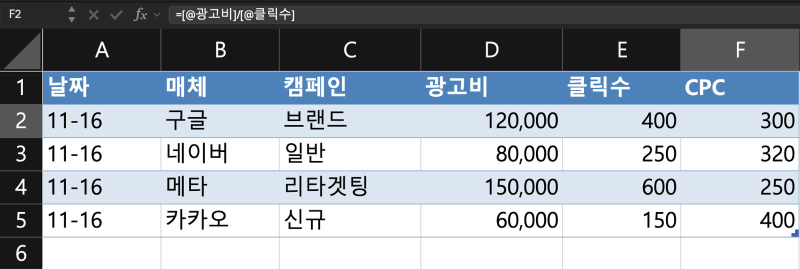 Source: an "Ads" table built with sample data in Microsoft Excel for Mac. Selecting F2 shows =[@광고비]/[@클릭수] — the Korean column names for Spend and Clicks — in the formula bar, and F3:F5 hold the same formula as a calculated column (screen in Korean).
To get a per-channel total outside the table, write something like =SUMIFS(Ads[Spend],Ads[Channel],"Google").
Just reading the formula tells you it means "the sum of Spend in the Ads table for rows where Channel is Google."
There are a few things to watch out for, which I'll cover separately in the notes section below.
3. How would this work for a weekly ad report?
Picture someone who downloads ad data by channel every Monday, stacks it on one sheet, and reports with a summary sheet and a pivot table. With a table, the workflow changes like this.
- Step 1: Turn the data range on the source sheet into a table and rename it "Ads."
- Step 2: Rewrite the SUMIFS on the summary sheet with structured references like
Ads[Spend]andAds[Channel]. - Step 3: Set the pivot table's source to the table name "Ads."
- Step 4: Paste next week's data into the leftmost cell right below the table's last row.
- Step 5: Just select [Refresh] on the pivot. The SUMIFS on the summary sheet include the new rows without any range edits.
The reason step 4 works is in the Resize a table by adding or removing rows and columns article. When you start typing in a cell below the last table row, the table expands to include that row, and when pasting, rows are added if you paste into the leftmost cell below the last table row. However, if the pasted data has more columns than the table, the extra columns don't become part of the table, so you need to widen it yourself with [Resize Table] on the [Table Design] tab.
Step 5 is also why the Create a PivotTable article calls tables a great data source. Rows added to a table are included automatically in the PivotTable when you refresh the data, and new columns appear in the PivotTable Fields list. Without a table, the article adds, you'd have to change the source range manually or use a dynamic named range formula.
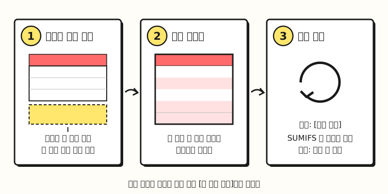 Paste below the table → the table expands automatically → refresh the pivot, and formulas stay as they are (figure labels in Korean).
If you're making a pivot for the first time, check the basics in my Excel pivot table post first, then connect this table as the source.
If you need a total line, turn on [Total Row] on the [Table Design] tab. According to the Total the data in an Excel table article, the total row uses the SUBTOTAL function, as in =SUBTOTAL(109,[Spend]), and the table overview article explains that rows hidden by a filter are excluded from the calculation by default.
If you filter down to "Google," the total row also becomes the Google total, so I'd recommend checking the filter state when you read numbers for a report.
※ Notes: what should I watch out for when using tables?
Tables are convenient, but some behaviors can catch you off guard if you don't know about them.
- Converting back to a range changes formulas: According to the Convert an Excel table to a range of data article, selecting [Convert to Range] in the [Tools] group on the [Table Design] tab keeps the table style formatting, but the sort and filter arrows disappear from the headers and structured references in formulas turn into regular cell references. Conversely, the structured references article notes that converting a range to a table doesn't automatically change existing formulas to structured references.
- Referencing a table in another file can cause #REF!: If the source workbook isn't open, the destination file can show #REF! errors, and opening the source resolves them. For reports that tie several files together, it's safer to keep the source in the same file. For errors like #REF!, see also my Excel formula errors post.
- If clicking inside a table inserts cell addresses: According to the structured references article, the "Use table names in formulas" check box under [File] → [Options] → [Formulas] controls this behavior. If it's cleared, selecting cells in a table inserts addresses like
D2:D40, so check that it's turned on. - Headers with special characters need double brackets: If a header contains special characters like % or $, you must wrap the whole header in an extra set of brackets, as in
Ads[[Conv Rate %]], and [ ] # ' @ need a single quotation mark (') in front. Keeping headers short and symbol-free makes formulas easier to write. - You can't move the header row when resizing: When you reselect the range with [Resize Table], the new range must overlap the original range.
- It's a different feature from "data tables": The table overview article points out that Excel tables are different from the data tables in the What-If Analysis commands. Mixing up "table" and "data table" when searching can bring up the wrong instructions.
The table overview article applies to Microsoft 365, Excel 2024 and 2021 (Windows and Mac), Excel 2019 and Excel 2016. So should you turn every sheet into a table?
When should I use a table, and when should I keep a range?
Based on the help articles, here are my own criteria.
- Better as a table: source data that grows every week or month, lists that feed pivots or SUMIFS and XLOOKUP, and rosters where several people add rows
- Better as a range: report layouts where you freely merge and decorate rows and columns, data referenced often from other files when you can't always keep the source file open, and files you'll hand to people who don't know structured references
- Splitting within one file: keep the source sheet as a table and the report sheet as a regular range, and have the report reference the table to get the benefits of both
Tables also help with lookup functions: write =XLOOKUP(A2,Ads[Campaign],Ads[Spend]) and the lookup range grows as rows are added to the source.
If the function itself is new to you, my VLOOKUP vs XLOOKUP post is a good companion.
Wrapping up
An Excel table looks like a formatting feature, but the point is that the range grows with your data and formulas read by column name. Turn source data that keeps growing into a named table and point your formulas and pivots at that name, and you'll spend less time fixing ranges every week. I'll share again if I notice anything different as I convert my report source sheets to tables. For detailed options, please refer to Microsoft's help articles.
FAQ
- What is the shortcut to create a table in Excel?
- In Excel for Windows, pressing Ctrl+T or Ctrl+L opens the [Create Table] dialog box. According to Microsoft's keyboard shortcuts article, it's Cmd+T or Ctrl+T on Mac and Ctrl+L in Excel for the web.
- What does @ mean in an Excel structured reference?
- It means "the same row as the formula." For example, [@Spend] is the Spend cell in that row. According to Microsoft's help, in tables with more than one data row Excel automatically replaces the #This Row specifier with the shorter @.
- What happens to formulas when I convert an Excel table back to a range?
- When you select [Convert to Range] on the [Table Design] tab, the table style formatting stays and structured references in formulas turn into regular cell references. The sort and filter arrows in the headers disappear as well.
- Are Excel tables and pivot tables the same feature?
- No. An Excel table is a range that holds source data, while a pivot table is a report that summarizes that data. If you use a table as a pivot source, rows added to the table are included automatically when you refresh the pivot.
More posts to explore
Posts that pair well with summarizing and connecting table data.
- What is an Excel pivot table? From meaning to creating and refreshing - Connect a table as the source and build a summary report
- Building pivot table reports with slicers and pivot charts - The next step after pivots: polishing your report
- VLOOKUP vs XLOOKUP - Lookup functions that connect values to other tables by column name